Artificial Intelligence for Cognition — Decoding Cognitive Conflict & Perception from EEG

Executive Summary & Scientific Context
This project represents my Bachelor’s Thesis (Treball de Final de Grau) in Artificial Intelligence at the Facultat d’Informàtica de Barcelona (FIB), Universitat Politècnica de Catalunya (UPC), completed under the academic supervision of Dr. Adrià Tauste Campo and Dr. Mireia Torralba Cuello (Department of Physics, UPC).
The work investigates whether non-invasive electroencephalography (EEG) recorded during onset binocular rivalry contains decodable information about perceptual conflict and conscious resolution on a single-trial basis. In binocular rivalry, incompatible visual stimuli (orthogonal red and green Gabor gratings) are presented dichoptically to each eye through a mirror stereoscope. Because the physical input remains conflicting while conscious perception fluctuates between one image, the other, or a mixed percept, this paradigm provides an experimental setting to isolate neural correlates of conscious perception from bottom-up sensory processing.
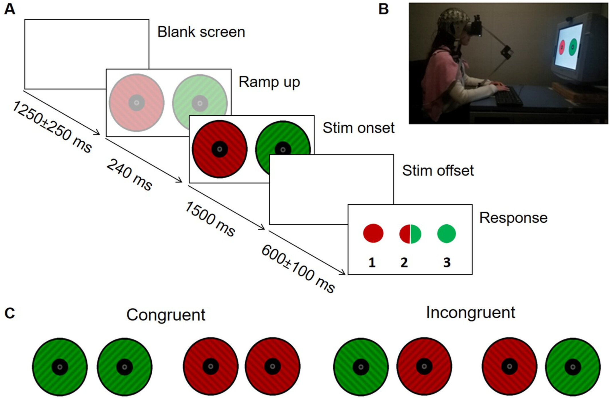 Figure 1: Onset binocular rivalry experimental timeline. Trials begin with a blank fixation, smooth fade-in ramp, stimulus presentation (main analysis window), variable jitter, and delayed response screen.
Two Core Classification Contrasts
To dissect conflict detection from motor execution and perceptual mixture, the study evaluates two binary classification tasks:
- Congruent vs. Incongruent-Pure (C vs. IP): Compares compatible binocular stimuli against incompatible stimuli where the observer reported complete single-color dominance. Because both classes involve identical single-color reports, this contrast tests the neural signature of interocular conflict while holding reporting behavior constant.
- Incongruent-Mixed vs. Incongruent-Pure (IM vs. IP): Evaluates two distinct perceptual outcomes under identical incompatible visual stimulation (unstable mixed percept vs. complete single-image dominance).
End-to-End Decoding Pipeline
60-electrode 10-10 montage, 500 Hz sampling rate, 0.5–45 Hz zero-phase bandpass filter, EOG artifact monitoring, and delayed-response epoch alignment (0–1.5 s).
Delaunay triangulation for sensor neighborhood graphs with 2D non-parametric Monte Carlo cluster-permutation testing to control family-wise error rate (FWER).
Structured hierarchy from hypothesis-driven baselines (FCz-theta, Oz-alpha) to Riemannian covariance, EEGNet, Spatio-Temporal GNNs, and Foundation Models.
Stratified Group K-Fold cross-validation preventing temporal leakage (autocorrelation r = 0.56) across session blocks, with fold-contained scaling.
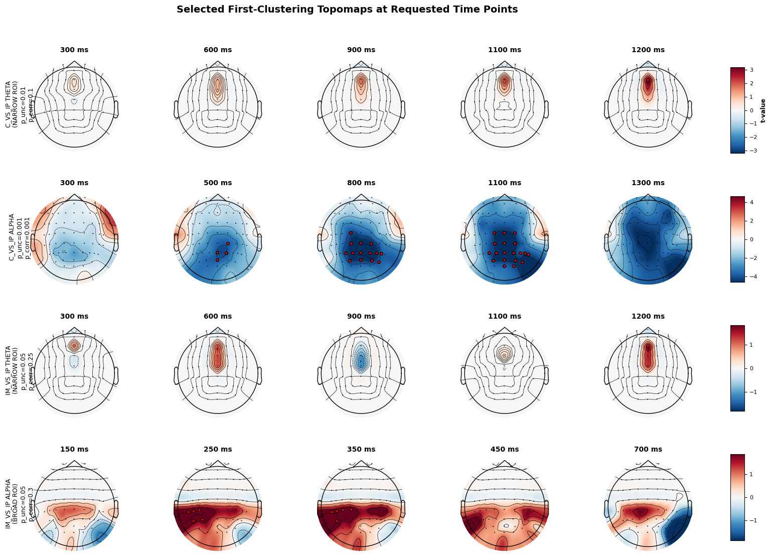 Figure 2: Two-dimensional cluster-based permutation test topomaps across representative time points, identifying broad posterior alpha suppression ($p_{\text{corrected}} = 0.0002$) and focal late fronto-medial theta effects ($p_{\text{corrected}} = 0.024$).
Machine Learning Architecture Hierarchy
The thesis compares 10 distinct modeling approaches under identical cross-validation constraints:
1. Classical & Riemannian Approaches
- Single-Feature Baselines: L2-regularized Logistic Regression on Hilbert envelope features (FCz-theta and Oz-alpha).
- Riemannian Covariance Decoding: Optimal Approximate Shrinkage (OAS) covariance matrices projected onto the Riemannian manifold tangent space at the Fréchet mean, paired with shrinkage Linear Discriminant Analysis (LDA).
- Cluster-Restricted SVC: Support Vector Classifiers trained directly on data-driven cluster summaries.
2. Deep Learning & Foundation Models
- EEGNet: Compact convolutional baseline (2,258 parameters, 100% trainable) using depthwise spatial filtering and separable convolutions.
- Spatio-Temporal Graph Neural Network (ST-GNN): 60-node sensor graph with Chebyshev spectral graph convolutions ($K=3$, 23,010 parameters, 100% trainable) combining spatial message passing with temporal convolutions.
- ST-EEGFormer: Transformer encoder backbone (25.8M parameters) adapted using rank-8 Low-Rank Adaptation (LoRA, $\alpha = 16$, 534k trainable parameters = 2.1%).
- LaBraM (Large Brain Model): Pre-trained patch-based EEG foundation model (5.8M parameters) adapted with LoRA adapters on attention/MLP layers (308k trainable parameters = 5.3%).
Experimental Results & Benchmark Comparison
The empirical findings from the final holdout evaluations across subjects are summarized below:
| Model Architecture | Parameter Scope | C vs. IP Balanced Acc (%) | IM vs. IP Balanced Acc (%) |
|---|---|---|---|
| Riemannian Covariance + LDA | Covariance Tangent Space | 58.7% ± 8.3% | 49.3% ± 6.1% |
| Experiment-Guided Classical ML | Feature Ensemble | 56.9% ± 8.1% | 50.9% ± 8.1% |
| SVC Cluster Features | RBF Kernel | 56.2% ± 6.3% | 52.7% ± 6.2% |
| Logistic Regression (Oz-alpha) | Single Feature | 53.6% ± 8.2% | 49.4% ± 8.0% |
| EEGNet (Agnostic) | 2.2k Params (100% Trainable) | 53.2% ± 8.2% | 49.5% ± 5.8% |
| ST-EEGFormer (LoRA) | 25.8M Params (2.1% Fine-Tuned) | 52.5% ± 8.3% | 50.7% ± 5.8% |
| ST-GNN (ChebConv) | 23k Params (100% Trainable) | 52.0% ± 7.3% | 51.4% ± 5.6% |
| LaBraM Adaptation (LoRA) | 5.8M Params (5.3% Fine-Tuned) | 51.9% ± 6.8% | 48.2% ± 9.6% |
| Logistic Regression (FCz-theta) | Single Feature | 49.6% ± 6.7% | 50.6% ± 8.6% |
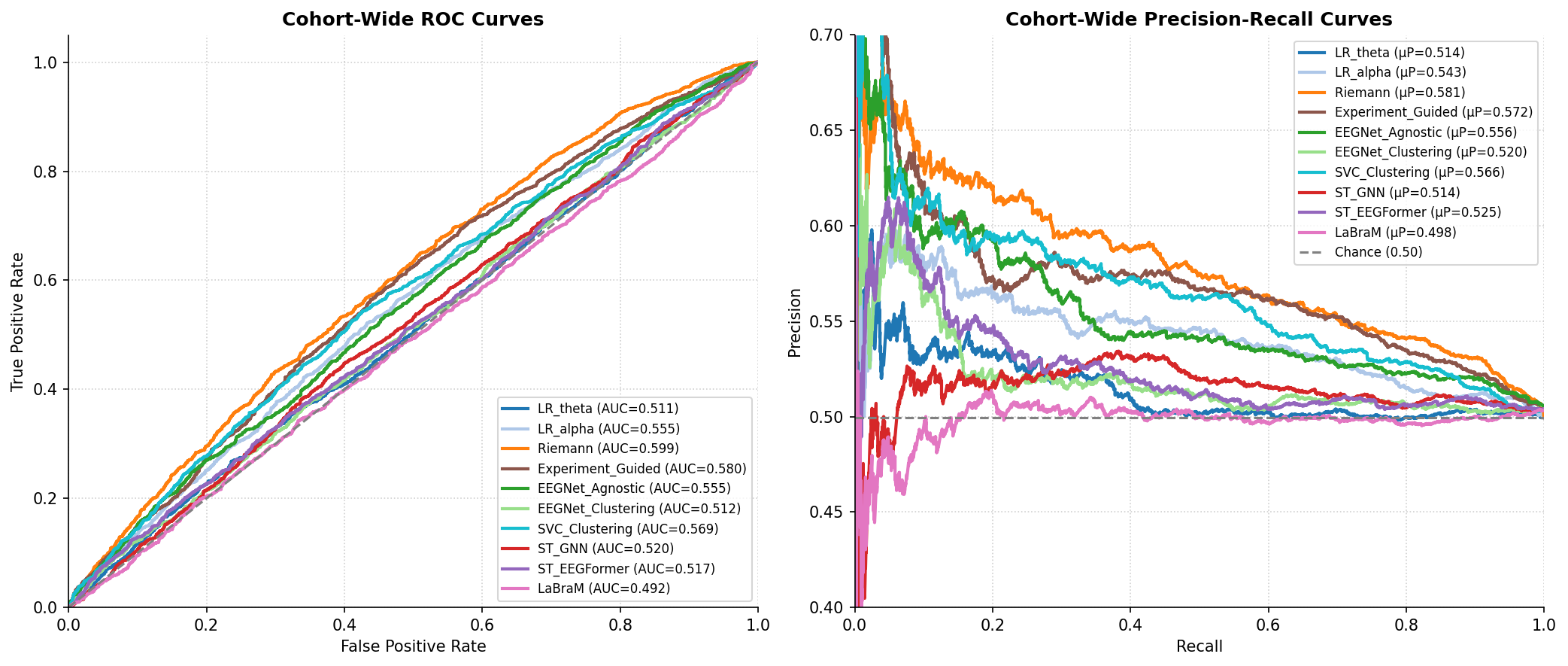 Figure 3: Cohort-wide Receiver Operating Characteristic (ROC) and Precision-Recall curves for C vs. IP, demonstrating clear above-chance separation led by Riemannian covariance.
Interpretability & Neuroscientific Diagnostics
Model interpretability was evaluated through Integrated Gradients (IG) on deep networks and weight projection on Riemannian classifiers, testing whether models relied on biologically plausible features rather than noise or session artifacts.
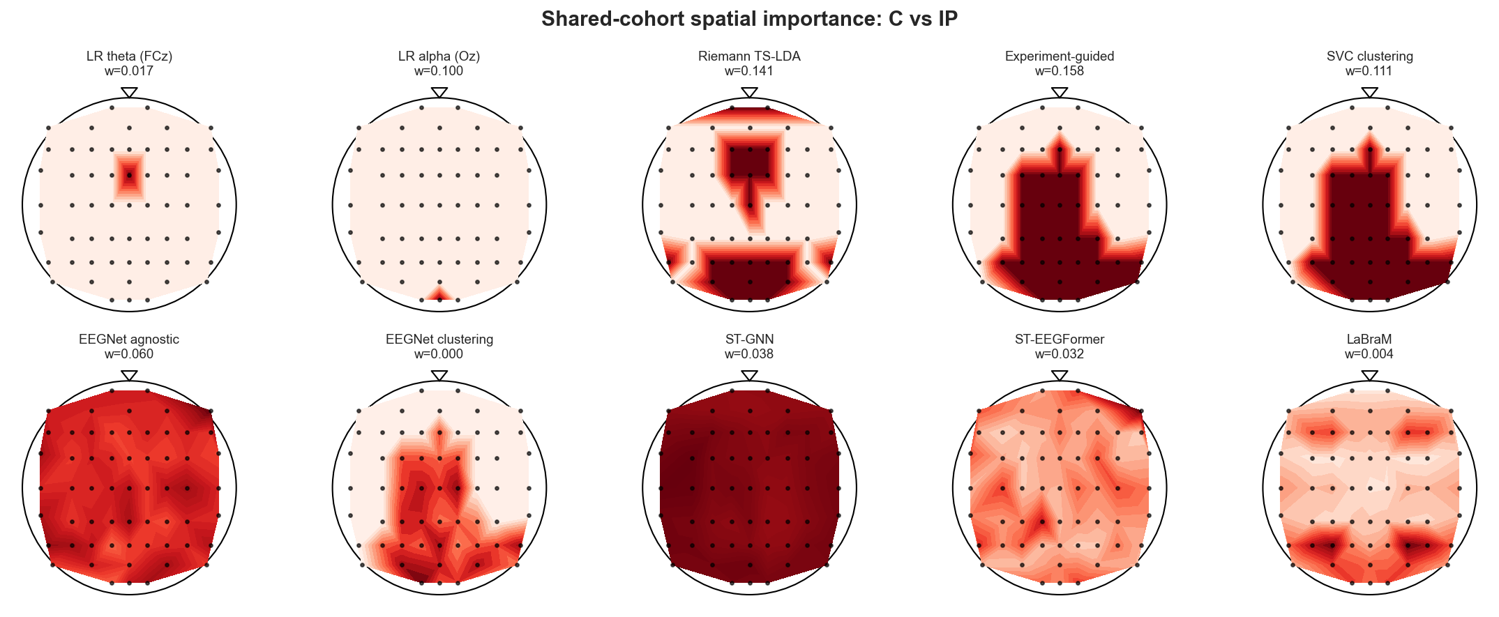 Figure 4: Spatial attribution topomaps across all 10 evaluated models for C vs. IP. Above-chance models consistently converge on broad posterior and parieto-occipital electrode regions.
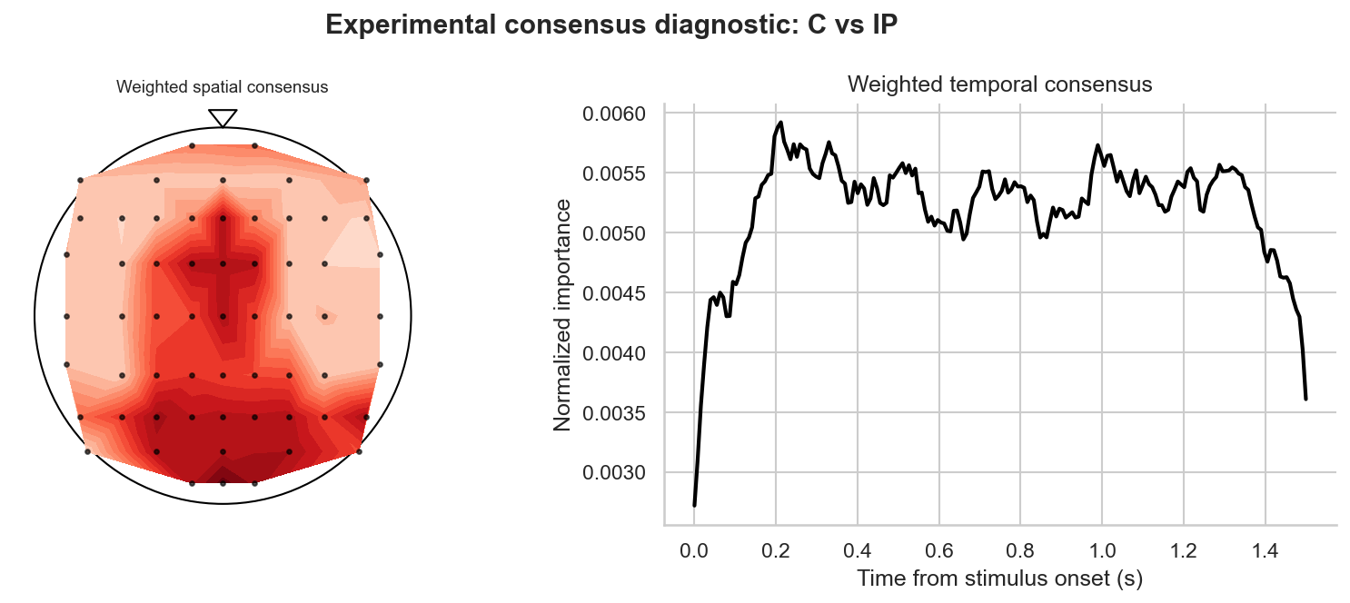 Figure 5: Experimental consensus diagnostic combining weighted spatial topographies and temporal attribution curves, showing sustained relevance from 400 ms through 1.2 s post-stimulus.
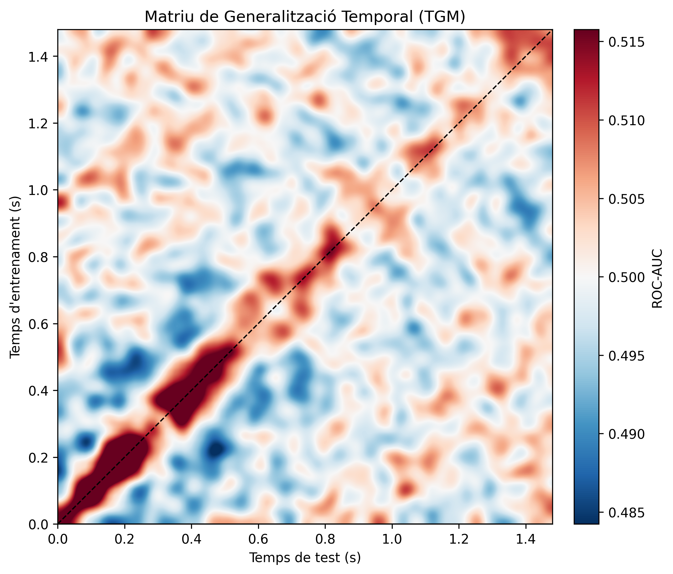 Figure 6: Temporal Generalization Matrix (TGM) showing that decodable information is dynamically localized in post-stimulus windows rather than persisting as a static trial-wide state.
Key Methodological Insights
- Why the Best Models Are Not the Largest Models: In low-SNR, subject-variable biomedical time series with modest trial counts, classical Riemannian covariance with strong geometric inductive biases outperforms 25M-parameter deep models. Larger models risk fitting to person-specific noise and session drift.
- Subject Identity Control: An auxiliary control experiment demonstrated that models could classify which subject produced a held-out trial with >98% accuracy, proving that EEG contains unique biometric signatures that necessitate strict grouped cross-validation to avoid leakage.
- Posterior Alpha vs. Fronto-Medial Theta: The decodable neural signature of perceptual conflict is dominated by broad posterior and occipital alpha modulations rather than isolated frontal theta rhythms.
- Reproducibility & Open Science: All data processing pipelines, modeling notebooks, and figure generation scripts are fully open-sourced on GitHub.